Tire model for longitudinal forces

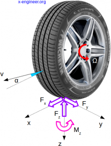
A vehicle’s tire must withstand forces and torques from several axes, depending on its driving state and direction of travel. In the contact patch of a tire from a driving axle, we can find longitudinal forces, side (lateral) forces, vertical forces and aligning torques.

The purpose of this article is to define a mathematical model of a tire, which can be used to calculate the longitudinal force in a tire (braking / traction) function of the vertical load of the tire. The mathematical model of a tire can be used for simulation purposes, mainly for development of wheel slip control strategies or for driving simulators (e.g. racing games).

The longitudinal force of the tire is generated when the vehicle is travelling in a straight line, during acceleration or braking. The side (lateral) wheel force is generated when the vehicle is changing direction, during cornering. The vertical tire force is given by the weight of the vehicle and depends on the dynamic behaviour of the suspension.

For a free rolling wheel, its longitudinal velocity is calculated as:

\[V_{x0} = r_{w} \cdot \Omega_{0}\]

When a torque is applied to the tire, either for acceleration or braking, a longitudinal slip occurs between the tire and the vehicle, calculated as:

\[ \begin{split}
k = \left\{\begin{matrix}
– \frac{V_{x0}-r_{w} \cdot \Omega}{V_{x0}} = – \frac{\Omega_{0}-\Omega}{\Omega_{0}} \text{, } a_{v}<0\\
\frac{r_{w} \cdot \Omega – V_{x0}}{r_{w} \cdot \Omega} = \frac{\Omega-\Omega_{0}}{\Omega} \text{, } a_{v}>0
\end{matrix}\right.
\end{split} \]

During braking, if the wheel is completely locked (Ω = 0), the tire slip will reach its minimum, -1. During acceleration, if the wheel is turning but the vehicle is at standstill (Ω₀ = 0), the tire slip reaches its maximum, 1.

The lateral tire slip is defined as the ratio between the lateral and longitudinal velocity of the wheel. This is equivalent with the tangent of the slip angle.

\[\tan(\alpha) = – \frac{V_{y}}{V_{x}}\]

The sign of the lateral tire slip has been chosen such that the lateral tire forces become positive when the tire slip angle is positive.

The lateral (side) and the longitudinal (brake/traction) tire forces depend on a great extent on the brake/traction slip and the lateral slip angle of the tire.

The aligning torque, also known as self aligning torque or aligning moment is the torque generated in a rolling tire, which tends to rotate the wheel around its vertical axis. When the tire side slip angle is non-zero, the aligning torque tends to steer the wheel in the direction of travel, hence the name self aligning torque.

The wheel camber angle is defined as the angle between the vertical axis of the wheel used for steering and the vertical axis of the vehicle when viewed from the front or rear.

The longitudinal, lateral tire forces and the aligning torque depend on four main parameters:

• tire longitudinal slip
• tire lateral slip
• wheel camber angle
• tire vertical load (force)

For simulation purposes, we need to have a mathematical expression of the tire forces function of the above parameters. One method of doing it is by using the Magic Formula equations. This method was developed by Hans B. Pacejka [1].

They equations are called “Magic Formula” because there is no particular physical basis for the structure of the equations, but they fit a wide variety of tire constructions and operating conditions. There are a set of equations and parameters for each: longitudinal tire force, lateral tire force and self-aligning moment. The parameters are determined as a best fit between experimental data and the tire model.

In this article we are going to focus only on the equations for the longitudinal tire force, for braking and acceleration.

Tire Model Magic Formula with Constant Parameters

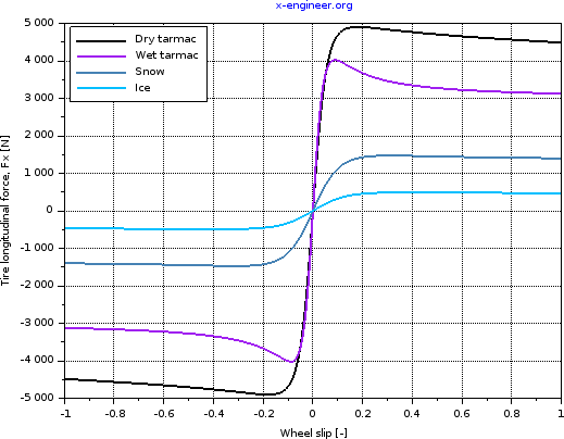
The simplest form of Pacejka’s Magic Formula has an equation with constant parameters:

\[F_{z} = F_{z} \cdot D \cdot \sin \left ( C \cdot \arctan \left \{ B \cdot k – E \cdot \left [ B \cdot k – \arctan(B \cdot k) \right ] \right \} \right )\]

As you can see, the longitudinal force F_x [N] depends only on two variables: the vertical load F_z [N] and the longitudinal tire slip k [-].

The dimensionless parameters B, C, D and E have constant values. These parameters are called:

• B: stiffness factor
• C: shape factor
• D: peak factor
• E: curvature factor

Depending on the surface of the road, these parameters have different values [2]:

Surface	B	C	D	E
Dry tarmac	10	1.9	1	0.97
Wet tarmac	12	2.3	0.82	1
Snow	5	2	0.3	1
Ice	4	2	0.1	1

The vertical tire load can be calculated function of the vehicle weight. If we consider that, for a 4-wheel vehicle, its weight is equally distributed between the wheels:

\[F_{z} = \frac{G_{v}}{4} = \frac{m_{v} \cdot g}{4}\]

Tire Model Load Dependent Parameters Magic Formula

A more realistic version of the Magic Formula has the parameters of the equation dependent on the tire longitudinal slip and vertical load [1].

\[F_{x} = D_{x} \cdot \sin \left ( C_{x} \cdot \arctan \left \{ B_{x} \cdot k_{x} – E_{x} \cdot \left [ B_{x} \cdot k_{x} – \arctan(B_{x} \cdot k_{x}) \right ] \right \} \right )+S_{Vx}\]

The values of the coefficients are given by the equations:

\[ \begin{split}
df_{z} &= \frac{F_{z}-F_{z0}}{F_{z0}}\\
\mu_{x} &= D_{x1} + D_{x2} \cdot df_{z}\\
S_{Hx} &= H_{x1} + H_{x2} \cdot df_{z}\\
S_{Vx} &= F_{z} \cdot (V_{x1} + V_{x2} \cdot df_{z})\\
K_{xk} &= F_{z} \cdot (K_{x1} + K_{x2} \cdot df_{z}) \cdot e^{K_{x3} \cdot df_{z}}\\
D_{x} &= \mu_{x} \cdot F_{z}\\
C_{x} &= C_{x1}\\
B_{x} &= \frac{K_{xk}}{C_{x} \cdot D_{x} + \epsilon_{x}}\\
k_{x} &= k + S_{Hx}\\
E_{x} &= (E_{x1} + E_{x2} \cdot df_{z} + E_{x3} \cdot df_{z}^{2}) \cdot (1 – E_{x4} \cdot \text{sgn}(k_{x}))
\end{split} \]

S_Hx and S_Vx are offsets to the tire slip and longitudinal force in the force-slip function, or horizontal and vertical offsets if the function is plotted as a curve. μ_x is the longitudinal load-dependent coefficient of friciton. ε_x is a very small number used to avoid division by zero as F_z approaches zero. df_z is the normalized change in vertical tire load.

A set of coefficients for the equations above can be found in [1]:

Cx1	Dx1	Dx2	Ex1	Ex2	Ex3	Ex4
1.685	1.21	-0.037	0.344	0.095	-0.02	0
Kx1	Kx2	Kx3	Hx1	Hx2	Vx1	Vx2
21.51	-0.163	0.254	-0.002	0.002	0	0

Tire Model for Longitudinal Forces Calculator

The generate the tire longitudinal force function of tire slip, use the calculator below. You can also tune the parameters in order to obtain the desired shape of the curves.

Fz [N]=
mv [kg]=	Cx1 [-]=	Dx1 [-]=	Dx2 [-]=
Ex1 [-]=	Ex2 [-]=	Ex3 [-]=	Ex4 [-]=
Kx1 [-]=	Kx2 [-]=	Kx3 [-]=	Hx1 [-]=
Hx2 [-]=	Vx1 [-]=	Vx2 [-]=	Calculate

Tire Model for Longitudinal Forces in Scilab

We can also use Scilab to generate the tire longitudinal forces. The first example is for the tire model with constant parameters.

clear()
clc()
clf()

// Tire model constant coefficients
B = [10 12 5 4];
C = [1.9 2.3 2 2];
D = [1 0.82 0.3 0.1];
E = [0.97 1 1 1];

// Vehicle parameters
mv = 2000;
g = 9.81;
Fz = (mv*g)/4;

// Plot setup parameters
surface = ["Dry tarmac" "Wet tarmac" "Snow" "Ice"];
colors = ["k" "purple" "steelblue" "deepskyblue"];

// Wheel slip
slip = [-1:0.01:1];

// Plot
for i=1:length(B)
    for j=1:length(slip)
        Fx(i,j) = Fz * D(i) * sin(C(i)*atan(B(i)*slip(j)-E(i)*(B(i)*slip(j)-atan(B(i)*slip(j)))));
    end
    plot(slip,Fx(i,:),"Color",colors(i),"LineWidth",2)
end
xgrid()
xlabel("Wheel slip [-]")
ylabel("Tire longitudinal force, Fx [N]")
title("x-engineer.org","Color","blue")
legend(surface,2)

By running the Scilab instructions above, we get the following graphical representation:

The second implementation in Scilab is for the Magic Formula with load dependent coefficients.

clear()
clc()
clf()

// Tire model load dependent coefficients
Cx1 = 1.685;
Dx1 = 1.21;
Dx2 = -0.037;
Ex1 = 0.344;
Ex2 = 0.095;
Ex3 = -0.02;
Ex4 = 0;
Kx1 = 21.51;
Kx2 = -0.163;
Kx3 = 0.254;
Hx1 = -0.002;
Hx2 = 0.002;
Vx1 = 0;
Vx2 = 0;
epsx = 1e-9;

// Vehicle and environmental parameters
mv = 2000;
g = 9.81;
Fz0 = (mv*g)/4;

// Wheel slip and tire vertical load
slip = [-1:0.01:1];
Fz = [500:500:Fz0];

// Tire longitudinal calculation
for i=1:length(Fz)
    dfz(i) = (Fz(i)-Fz0)/Fz0;
    mux(i) = Dx1 + Dx2 * dfz(i);
    SHx(i) = Hx1 + Hx2 * dfz(i);
    SVx(i) = Fz(i) * (Vx1 + Vx2 * dfz(i));
    Kxk(i) = Fz(i) * (Kx1 + Kx2 * dfz(i)) * exp(Kx3 * dfz(i));
    Dx(i) = mux(i) * Fz(i);
    Cx(i) = Cx1;
    Bx(i) = Kxk(i) / (Cx(i) * Dx(i) + epsx);
    for j=1:length(slip)
        kx(i,j) = slip(j) + SHx(i);
        Ex(i,j) = (Ex1 + Ex2 * dfz(i) + Ex3 * dfz(i)^2) * (1 - Ex4 * sign(kx(i,j)));
        Fx(i,j) = Dx(i)*sin(Cx(i)*atan(Bx(i)*kx(i,j)-Ex(i,j)*(Bx(i)*kx(i,j)-atan(Bx(i)*kx(i,j)))))+SVx(i);
    end
    plot(slip,Fx(i,:),"LineWidth",1)
    xstring(0.15,max(Fx(i,:)),strcat(["Fz = " string(Fz(i)) " N"]));
end

// Pot setup
xgrid()
xlabel("Wheel slip [-]")
ylabel("Tire longitudinal force, Fx [N]")
title("x-engineer.org","Color","blue")

By running the Scilab instructions above, we get the following graphical representation:

Tire Model for Longitudinal Forces in Xcos

For simulation purposes of chassis dynamics, we might need to have the Magic Formula implemented in Xcos. The following model implements both constant and load dependent parameters model using Xcos block diagram.

The longitudinal tire slip is generated using an interpolation map, based on the simulation time.

The Constant Coefficients Xcos model is implemented as:

The constant parameters need to be loaded in the Scilab workspace before the simulation is run.

The Load Dependent Coefficients Xcos model is implemented using a C block:

By running the simulation and doing post-processing of the longitudinal tire force saved in the Scilab workspace, we get the following shapes:

Conclusion

The Pacejka’s Magic Formula tire models are widely used in professional vehicle dynamics simulations, and racing car games, as they are reasonably accurate, easy to program, and solve quickly. Each tire is characterised by a number of coefficients (10 – 20) for each important force that it can produce at the contact patch, typically lateral and longitudinal force, and self-aligning torque, as a best fit between experimental data and the model. These coefficients are then used to generate equations showing how much force is generated for a given vertical load on the tire, camber angle and slip angle.

References:

[1] Hans B. Pacejka, Tyre and Vehicle Dynamics, Delft University of Technology, 2002.
[2] https://uk.mathworks.com/help/physmod/sdl/ref/tireroadinteractionmagicformula.html