Modeling and simulation of a vehicle with automatic transmission

3. Plant model: Engine

The engine used for the simulation example is a Mercedes 5.0 litre V8, with the following performance parameters:

• maximum engine power @ engine speed [kW@rpm]: 225 @ 5600
• maximum engine torque @ engine speed Nm@rpm]: 460 @ 3000-4250

The engine torque is mapped, function of the accelerator (throttle) position and engine speed. Only the full load data points are matched against the real engine torque output. The part load torque values are extrapolated from the full load points.

Engine torque [Nm]		Engine speed [rpm]
		1000	1500	2000	2500	3000	3500	4000	4500	5000	5500	6000
Accelerator pedal (throttle) position [%]	0	0	-25	-50	-71	-89	-105	-116	-128	-139	-150	-161
	20	241	155	93	57	30	6	-16	-36	-53	-68	-81
	30	283	236	195	163	137	116	99	85	75	67	61
	40	314	326	334	328	308	275	238	199	168	150	140
	50	329	346	361	371	373	365	346	316	276	230	187
	60	349	365	378	387	396	398	384	357	322	284	246
	70	359	382	400	411	417	417	409	396	370	334	299
	80	367	399	424	436	439	440	438	426	400	368	332
	90	373	408	435	448	451	451	449	436	414	385	349
	100	377	414	443	456	460	460	460	450	427	402	366

In graphical form, the engine torque output at full load and part loads looks like:

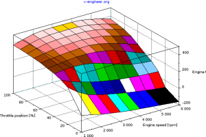Image: Engine torque map – 3D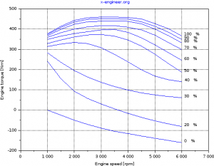

Image: Engine torque map – 2D

The engine provides positive torque during acceleration phases and negative (braking) torque in the overrun phases. The engine is modelled as a single inertia lumped parameters and a torque map.

The governing differential equation of the engine model is:

\[J_{e} \frac{d \omega_{e} }{dt} = T_{e}-T_{i} \tag{1}\]

From equation (1) we can calculate the engine speed as:

\[\omega_{e} = \frac{1}{J_{e}} \int (T_{e}-T_{i}) dt \tag{2}\]

To convert the engine speed from [rad/s] into [rpm], we use the following expression:

\[N_{e} = \frac{30 \cdot \omega_{e}}{\pi} \tag{3}\]

The engine power can be calculated as:

\[P_{e} = \frac{T_{e} \cdot \omega_{e}}{1000} \tag{4}\]

Equations (2), (3) and (4) are used to define the Xcos block diagram for engine simulation.

The calculated engine speed is limited to a maximum and a minimum value. The minimum value is considered the idle speed of the engine.

Inputs

Name	Value	Description
ImplTq_Nm	–	Impeller torque [Nm]
AccrPedlPosn_prc	–	Accelerator pedal position [%]

Parameters

Name	Value	Description
EngImplJ_kgm2_C	0.08	Engine and impeller inertia [kg·m2]
EngMaxN_rpm_C	7000	Maximum engine speed [rpm]
EngMinN_rpm_C	1000	Minimum engine speed [rpm]
EngN_rpm_X	(table)	Engine speed axis [rpm]
AccrPedlPosnEng_prc_Y	(table)	Accelerator pedal position axis [%]
EngTq_Nm_Z	(table)	Engine torque map [Nm]

Outputs

Name	Value	Description
EngN_rpm	–	Engine speed [rpm]