Anti-lock braking system (ABS) modeling and simulation (Xcos)

Mathematical modeling and simulation bring significant benefits in terms of understanding the braking phenomena and the impact of different parameters on the braking performance of a vehicle.

Anti-lock braking systems (ABS) are meant to control the wheel slip in order to maintain the friction coefficient close to the optimal value. Wheel slip is defined as the relative motion between a wheel (tire) and the surface of the road, during vehicle movement. Wheel slip occurs when the angular speed of the wheel (tire) is greater or less compared to its free-rolling speed.

In order to simulate the braking dynamics of a vehicle, we are going to implement simplified mathematical models (quarter-car model) for both vehicle and wheel. Also, a simplified ABS controller is going to be implemented in order to emulate the braking torque in slip conditions.

Vehicle model

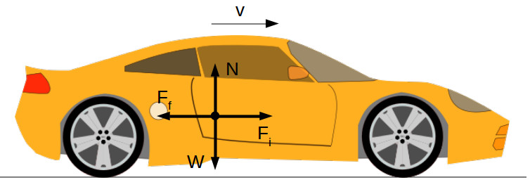
If we consider a vehicle moving in a straight direction under braking conditions, we can write the equations of equilibrium:

• for horizontal direction:

\[F_f = F_i \tag{1}\]

where:

F_f [N] – is the friction force between wheel and ground
F_i [N] – is the inertial force of the vehicle

• for vertical direction:

\[N = W \tag{2}\]

where:

N [N] – normal force (road reaction)
W [N] – vehicle weight

We can write the expressions of the friction force as:

\[F_f = \mu \cdot N \tag{3}\]

where μ [-] the friction coefficient between wheel and road.

The vehicle’s weight is:

\[W = m_v \cdot g \tag{4}\]

Replacing (2) and (4) in (3) gives the expression of the friction force as:

\[F_f = \mu \cdot m_v \cdot g \tag{5}\]

where:
m_v [kg] – is the total vehicle mass
g [m/s²] – is the gravitational acceleration

The inertia force is the product between the vehicle mass m_v [kg] and vehicle acceleration a_v [m/s²]:

\[F_i = m_v \cdot a_v = m_v \cdot \frac{dv_v}{dt} \tag{6}\]

where v_v [m/s] is the vehicle speed.

From equations (1), (5) and (6) we can extract the expression of the vehicle acceleration:

\[\bbox[#FFFF9D]{\frac{dv_v}{dt}=\frac{1}{m_v} \cdot (\mu \cdot m_v \cdot g)} \tag{7}\]

Vehicle speed is obtained by integration of equation (7).

Wheel model

During braking, through the braking system, the driver applies a braking torque T_b [Nm] to the wheels. The friction force F_f [N] between the wheel and road creates an opposite torque with the wheel radius r_w [m].

For simplification, we are going to consider that the wheel is rigid and the normal force (road reaction) passes through the wheel hub, therefore doesn’t add an additional torque.

We can write the equation of equilibrium for the wheel as:

\[T_b – F_f \cdot r_w – J_w \cdot \frac{d \omega_w}{dt}=0 \tag{8}\]

where:

J_w [kg·m²] – is the wheel’s moment of inertia
ω_w [rad/s] – is the angular speed of the wheel

From equation (8) we can extract the expression of the wheel acceleration:

\[\bbox[#FFFF9D]{\frac{d \omega_w}{dt} = \frac{1}{J_w} \cdot (T_b – F_f \cdot r_w)} \tag{9}\]

Wheel speed is obtained by integration of equation (9).

Wheel slip

The ABS system has to control the wheel slip s [-] around an optimal target. The wheel slip is calculated as:

\[s = 1 – \frac{\omega_w}{\omega_v} \tag{10}\]

where ω_v [rad/s] is the equivalent angular speed of the vehicle, equal with:

\[\omega_v = \frac{v_v}{r_w} \tag{11}\]

where v_v [m/s] is the vehicle speed.

Friction coefficient

The friction coefficient between wheel and road depends on several factors, like:

• wheel slip
• vehicle speed
• the type of the road surface
• environmental conditions (humidity, temperature, etc.)

For our simulation purpose, we are going to take into account only the variation of the friction coefficient function on the longitudinal wheel slip.

During braking, if the wheel slip is 100 % the wheel is locked but the vehicle is still moving. At 0 % slip, the wheel and vehicle have exactly the same speed.

The optimum friction coefficient (highest value) is obtained when the wheel slip is around 20 %. As you can see, the friction coefficient curve is split into two areas:

• stability zone: where the friction coefficient increases with the wheel slip increase
• unstable zone: where the friction coefficient decreases with the wheel slip increase

If the wheel slip enters the unstable area, the friction coefficient will decrease and the wheel will lock causing skid and vehicle instability.

For this particular example, the ABS systems will have to keep the wheel slip around 20 %, where friction coefficient has the highest values.

The friction coefficient can be expressed as an empirical function, where the wheel slip is a function argument:

\[\mu(s) = A \cdot \left ( B \cdot \left ( 1 – e^{-C \cdot s}\right ) – D \cdot s \right ) \tag{12}\]

where:

s [-] – is the wheel slip
A, B, C, D [-] – are empirical coefficients

Depending on the value of the coefficients A, B, C and D, the empirical formula (12) can be used to represent the friction coefficient for different road types/states.

	Road type/state
	dry concrete	wet concrete	snow	ice
A	0.9	0.7	0.3	0.1
B	1.07	1.07	1.07	1.07
C	0.2773	0.5	0.1773	0.38
D	0.0026	0.003	0.006	0.007

Using a Scilab script we can plot the variation of the friction coefficient functio of slip, for different road conditions.

A = [0.9 0.7 0.3 0.1];
B = [1.07 1.07 1.07 1.07];
C = [0.2773 0.5 0.1773 0.38];
D = [0.0026 0.003 0.006 0.007];

slip_x = [0:100];
colors = ["b","r","g","k"]

for i=1:length(A)
    for j=1:length(slip_x)
        miu_y(i,j) = A(i)*(B(i)*(1-exp(-C(i)*slip_x(j)))-D(i)*slip_x(j));
    end
    figure(1)
    hf=gcf();
    hf.background=8;
    plot(slip_x,miu_y(i,:),colors(i))
end
ha=gca();
xlabel("Wheel slip [%]","FontSize",2)
ylabel("Friction coefficient, miu [-]","FontSize",2)
xgrid();
title("x-engineer.org","FontSize",2)
legend("dry concrete","wet concrete","snow","ice")

From the image above we can see that the maximum value of the friction coefficient decreases sharply for a road covered by snow or ice. Even if the value of the friction coefficient is not significantly lower for 100 % slip, preventing wheel lock improves vehicle maneuverability (steering).

Model parameters

For our simulation example, we are going to use a vehicle with the following parameters:

Symbol	Unit	Value	Description
mv	kg	1200	total vehicle mass
Jw	kg·m2	0.01	wheel inertia
rw	m	0.28	wheel radius
v0	m/s	28	initial vehicle speed
vmin	m/s	1.4	minimum vehicle speed for slip control active
g	m/s2	9.81	gravitational acceleration

There are also a couple of other parameters used by the slip controller and other settings:

Symbol	Unit	Value	Description
K	–	1000	hydraulic system amplification factor
T	s	0.01	time constant to simulate braking system inertia
Tbmax	Nm	2000	maximum braking torque applied to the wheels
ε	–	2.2204·10-16	division by zero protection constant
ON	–	1 or 0	logic variable for activation/deactivation of the slip controller
road type	–	1, 2, 3 or 4	constant for road type setting

Xcos block diagram

The vehicle and wheel model used for the simulation is known in the literature as a quarter-car model. This means that a quarter of the vehicle mass is considered with only one wheel. Also, only the longitudinal vehicle dynamics is considered, disregarding the impact of the suspension system.

Before starting modeling the Xcos block diagram, we need to define and load in the Scilab workspace the model parameters, which are defined in a Scilab script:

mv = 1200;
Jw = 0.01;
rw = 0.28;
v0 = 28;
vmin = 1.4;
g = 9.81;
K = 1000;
T = 0.01;
Tbmax = 2000;
eps = 2.2204e-16;
ON = 1;
roadType = 1;

The high level Xcos diagram contains the main components (as user defined functions) and the interfaces between them. All the outputs of each component are fed into Goto blocks which are merged in a MUX block.

The multiplexed outputs are saved in the Scilab workspace using a To workspace block sampled at 0.01 s.

Further, we are going to describe in detail each component and its input and output signals

VEHICLE

The vehicle model is implementing equation (7). Since we are using a quarter-car model, the total weight of the vehicle is divided by 4, assuming equal distribution on each wheel.

The input of the model is the friction coefficient μ [-], which is function of the wheel slip.

The integrator block has the initial value v0 and it is saturated to maximum 1000 m/s and minimum 0 m/s. To avoid numerical instabilities in the wheel slip calculation, the saturation block limits the minimum vehicle speed at 0.001 m/s keeping the same maximum limit.

The distance covered by the vehicle is calculated by integration of the vehicle speed.

Outputs:

• friction force F_f [N]
• vehicle speed v_v [m/s]
• equivalent vehicle speed ω_v [rad/s]
• vehicle distance d_v [m]

WHEEL

The wheel model is implementing equation (9). The wheel speed (angular) ω_w [rad/s] integrator is initialized with v0/rw [rad/s] and saturated to maximum 1000 rad/s and minimum 0 rad/s. The linear wheel speed v_w [m/s] is obtained by multiplying the angular speed with the wheel radius r_w [m]. The distance covered by the wheel d_w [m] is obtained by integrating the linear speed.

Inputs:

• braking torque T_b [Nm]
• friction force F_f [N]

Outputs:

• angular wheel speed ω_w [rad/s]
• linear (tangential) wheel speed v_w [m/s]
• wheel distance d_w [m]

SLIP

Wheel slip is calculated using equation (10). When the vehicle speed is zero, to avoid division by zero, the ε constant is used as a denominator. The calculated slip value is further saturated to a maximum 1 and minimum 0.

Inputs:

• wheel angular speed ω_w [rad/s]
• vehicle angular speed ω_v [rad/s]

Outputs:

• wheel slip s [-]

FRICTION

The friction coefficient diagram is implementing four variants of the equation (12), each one for a different road state. The mathematical expressions of the friction coefficient expect as argument the wheel slip in [%] therefore s [-] is multiplied with 100 using a Gain block. The road dependent friction coefficient is selected using a Dynamic index block, which is controlled by the variable roadType. The friction coefficient is saturated between a minimum 0 and a maximum 1.

Inputs:

• wheel slip s [-]

Outputs:

• friction coefficient μ [-]

CONTROL

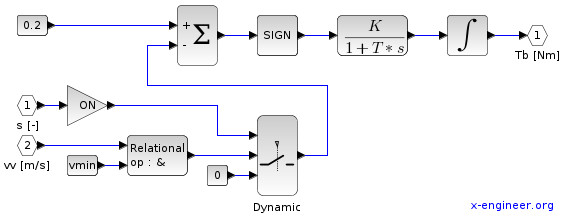
The slip controller is fairly simple. It’s a bang-bang type controller, reacting on wheel slip feedback, emulating the ABS controller. As discussed in the friction coefficient section above, the maximum value of the friction coefficient is obtained around a slip of 20 %. Therefore we set a target (reference) slip of 0.2. A slip error is calculated by subtracting the actual slip from the target slip. To avoid the action of the controller at low speeds, the actual slip s [-] is only used when the vehicle speed is higher than vmin [m/s].

Depending on the slip error, the SIGN block will output:

• 1, if s > 0
• 0, if s == 0
• -1, if s < 0

The hydraulic system is modeled as a first order transfer function, with the amplification factor K and time constant T. The output of the transfer function is the brake torque T_b [Nm] which is accumulated over time by the integrator. The integrated torque is limited between 0 Nm and Tbmax [Nm].

Inputs:

• wheel slip s [-]
• vehicle speed v_v [m/s]

Outputs:

• braking torque T_b [Nm]

Simulation results

The simulation scenario is braking from an initial speed of v₀ [kph] until a complete vehicle stop, with the driver braking heavily.

There are two test cases:

• without ABS: the slip controller is disabled by setting the parameters ON = 0
• with ABS: the slip controller is enabled by setting the parameters ON = 1

The Xcos simulation will is run for 20 s.

The simulation results are described below, on the left side the vehicle is braking without ABS, on the right side with ABS.

Image: Wheel braking torque (without ABS)

Image: Wheel braking torque (with ABS)

When the ABS system is disabled, the braking torque ramps up to maximum value (2000 Nm) in just 2 s. With the ABS system active (slip control), the braking torque is modulated to keep the wheel slip around target value (20 %). When the wheel speed is less than the minimum value (1.4 m/s), the braking torque is not controlled anymore and it increases to maximum value.

Image: Wheel slip (without ABS)

Image: Wheel slip (with ABS)

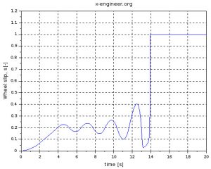
When the ABS system is deactivated, as the torque increases, the wheel slip climbs up rapidly towards 1 (wheel lock). With the ABS system active, the wheel slip is regulated around 20 %. Since the wheel slip control is not active below 1.4 m/s, the wheel locks and the slip goes to 1.

Image: Wheel friction coefficient (without ABS)

Image: Wheel friction coefficient (with ABS)

Without ABS, since the wheel locks, the friction coefficient decreases to approx. 0.7. With the slip control active (with ABS), the friction coefficient is kept near maximum value 0.9. This gives higher friction force between wheel and road, which will help stop the vehicle faster.

Image: Wheel and vehicle speed (without ABS)

Image: Wheel and vehicle speed (with ABS)

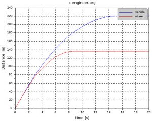
When the ABS system is deactivated, the wheel locks before the vehicle comes to complete stop. Also, it is noticeable that the gradient of the speed changes after the wheel lock. This happens because the friction force becomes smaller and the braking distance increases.

With the ABS active, the wheel is prevented from locking. Having the wheel slip around optimal value provides a higher friction force between wheel and road thus a shorter braking distance (the vehicle comes to a complete stop faster).

Image: Wheel and vehicle distance (without ABS)

Image: Wheel and vehicle distance (with ABS)

When braking without ABS, the braking distance for the vehicle to come to a complete stop is around 220 m. When the wheel slip is controlled (ABS active), the braking distance is decreased with around 10 m, which is quite significant.

From the simulation we can see that the ABS system is reducing the braking distance of a vehicle. Also, preventing wheel lock allows the drive to steer and avoid road hazards.

The source code for the simulation plots is in the Scilab script below.

Tb=sOut.values(:,1);
mu=sOut.values(:,2);
s=sOut.values(:,3);
Ff=sOut.values(:,4);
vv=sOut.values(:,5);
wv=sOut.values(:,6);
dv=sOut.values(:,7);
ww=sOut.values(:,8);
vw=sOut.values(:,9);
dw=sOut.values(:,10);
time=sOut.time;

figure(1)
hf=gcf();
hf.background=8;
ha=gca();
plot(time,Tb)
xlabel("time [s]","FontSize",2)
ylabel("Braking torque, Tb [Nm]","FontSize",2)
xgrid();
title("x-engineer.org","FontSize",2)

figure(2)
hf=gcf();
hf.background=8;
ha=gca();
plot(time,s)
ha.data_bounds = [0,0;max(time),1]
xlabel("time [s]","FontSize",2)
ylabel("Wheel slip, s[-]","FontSize",2)
xgrid();
title("x-engineer.org","FontSize",2)

figure(3)
hf=gcf();
hf.background=8;
ha=gca();
plot(time,mu)
xlabel("time [s]","FontSize",2)
ylabel("Friction coefficient, miu [-]","FontSize",2)
xgrid();
title("x-engineer.org","FontSize",2)

figure(4)
hf=gcf();
hf.background=8;
ha=gca();
plot(time,vv*3.6)
plot(time,vw*3.6,"r")
xlabel("time [s]","FontSize",2)
ylabel("Speed [kph]","FontSize",2)
xgrid();
title("x-engineer.org","FontSize",2)
legend("vehicle","wheel",1)

figure(5)
hf=gcf();
hf.background=8;
ha=gca();
plot(time,dv)
plot(time,dw,"r")
xlabel("time [s]","FontSize",2)
ylabel("Distance [m]","FontSize",2)
xgrid();
title("x-engineer.org","FontSize",2)
legend("vehicle","wheel",1)

figure(6)
hf=gcf();
hf.background=8;
ha=gca();
plot(time,wv)
plot(time,ww,"r")
xlabel("time [s]","FontSize",2)
ylabel("Angular speed [rad/s]","FontSize",2)
xgrid();
title("x-engineer.org","FontSize",2)
legend("vehicle","wheel",1)

Don’t forget to Like, Share and Subscribe!