How to plot a vector field

Vector field plots are linked to differential equations. When we solve a differential equation, we don’t get a particular (unique) solution, we get a general solution, which is basically a family of particular solutions.

For an easier understanding let’s jump directly to an example. Suppose we have the differential equation:

\[\frac{dy}{dx}=x\]

This is a separable first order differential equation, because we can write it with all the y‘s on one side of the equal sign, and all the x‘s on the other side, like this:

\[dy=x \cdot dx\]

With other words, we have separated the y‘s from the x‘s. We solve it by integrating both sides of the equation:

\[\int dy = \int x \cdot dx\]

The solution is straightforward:

\[y = \frac{x^2}{2}+C\]

where C is a constant.

Notice that the solution in not unique (particular) but general, because the constant C can take any value (real number). This means that our differential equation can have as many solutions as possible values of the constant C.

Using vector field plots we can see the representation of all the solutions of a linear differential equation between fixed boundaries.

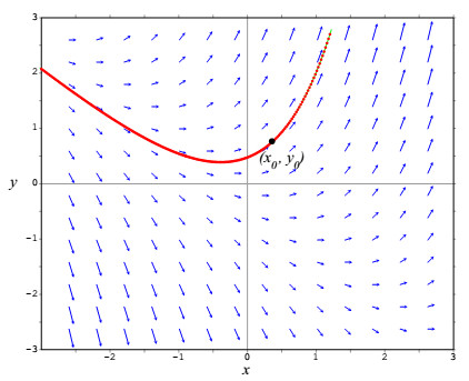
In the image above we can see the vector field plot for the differential equation:

\[\frac{dy}{dx}=y+x\]

The small blue arrows (vectors) indicate the tendency (shape) of the solutions of the differential equation between the boundaries of the plot. The red line represents a particular solution of the differential equation.

By drawing the vector field plot we will know, before solving the differential equation, how the solution will look like in terms of the shape of the curve.

The question is: how do we draw the vector field plot having only the differential equation?

We will use the same differential equation, which we solved previously, as example:

\[\frac{dy}{dx}=x\]

First we need to recall that we can define the equation of a line y = f(x) having one point (x₀, y₀) and the slope m:

\[y-y_0 = m \cdot (x – x_0)\]

For small values of x, the slope m is the derivative of the function:

\[m=\frac{dy}{dx}\]

By replacing the equation of the slope in the line equation, we get:

\[y-y_0 =\frac{dy}{dx} \cdot (x – x_0)\]

All the vectors in the field plot are small lines defined by the equation above for different values of the start point (x₀, y₀) and slope dy/dx.

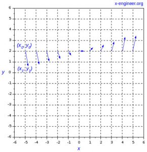
In the table below we are going to calculate the points which define the vectors.

Step 1. Choose the value of x₀.

Step 2. Choose the value of y₀.

Step 3. The value of the slope is equal with the value of the differential equation. In our case, the differential equation is equal to x, so the value of the slope is the same as the value of the point x₀.

\[m = \frac{dy}{dx} = x = x_0\]

Step 4. We choose the point x₁ equal to the point x₀ plus an offset (0.3).

\[x_1 = x_0 + 0.3\]

Step 5. Calculate the value of the point y₁ using the equation of the line:

\[y_1 = m(x_1-x_0)+y_0\]

Step 6. Draw line between (x₀, y₀) and (x₁, y₁)

All the above steps are summarized in the table below.

Step	1	2	3	4	5	6
Vector	x0	y0	m	x1	y1	Draw line
1	-5	2	-5	-4.7	0.6
2	-4	2	-4	-3.7	0.8
3	-3	2	-3	-2.7	1.1
4	-2	2	-2	-1.7	1.4
5	-1	2	-1	-0.7	1.7
6	0	2	0	0.3	2
7	1	2	1	1.3	2.3
8	2	2	2	2.3	2.6
9	3	2	3	3.3	2.9
10	4	2	4	4.3	3.2
11	5	2	5	5.3	3.5

After we calculate all the end points (x₁, y₁), we can draw each vector line:

The process can be repeated for different values of y.

In order to make the calculations faster we can use the Scilab script below:

// Clear Scilab console and all variables
clc
clear

// Define differential function
deff('f=dydx(x,y)','f=x');

// Define variable range
xmin = -5; xmax = 5; x=xmin:xmax;
ymin = -5; ymax = 5; y=ymin:ymax;

// Graphic window setup
figure(0);
hf=gcf();
hf.axes_size = [480,480];
hf.background = 8;
ha=gca();
ha.grid=[33,33];

// Vector field plot
for i=1:length(x)
   for j=1:length(y)
      m = dydx(x(i),y(j));
      offset=0.3;
      xl = x(i)+offset; 
      yl = m*(xl-x(i))+y(j);
      plot([x(i) xl],[y(j) yl]);
   end
end

// Rescale the axes of the figure
ha.data_bounds = [xmin-1 ymin-1;xmax+1 ymax+1];

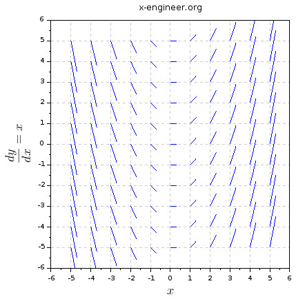
The differential equation is defined as a function, using the embedded Scilab function deff(). After running the script, we get the vector field plot for the specified x and y boundaries.

To check our statement, that the vector field plot of a differential equation is the family of all particular solutions within specified boundaries, we are going to plot on the same figure the line plot of the general solution y(x) for C = -2, -1, 0, 1, 2.

\[y(x) = \frac{x^2}{2}+C\]

As you can see, each of the curves for the particular solutions follow the direction of the vector field.

In order to check if our Scilab script is generating the correct vector field plot, we are going to use it for two more differential equations, which have a defined vector field plot.

\[\frac{dy}{dx}=y+x\]

The vector field plot of this differential equation can be found here.

Change the function definition in the Scilab script:

deff('f=dydx(x,y)','f=y+x');

and run the script.

On the left image is the vector field plot specified at the source above, on the right side, we have the vector field plot generated by the Scilab script.

Image: Vector field plot for the differential equation dy/dx = y + x

Image: Scilab vector field plot for the differential equation dy/dx = y + x

As you can see, the direction of the vector field are the same in both plots.

Repeat the steps above for the function:

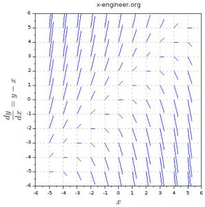
\[\frac{dy}{dx}=y-x\]

The vector field plot of this differential equation can be found here.

Image: Vector field plot for the differential equation dy/dx = y – x

Image: Scilab vector field plot for the differential equation dy/dx = y – x

Again, the Scilab script is generation the same vector field plot.

Use the script to generate vector field plots for different differential equations. Then solve the equations and see if the line plot for a particular solution is matching the direction of the vector field.

For any questions, observations and queries regarding Scilab variables use the comment form below.

Don’t forget to Like, Share and Subscribe!