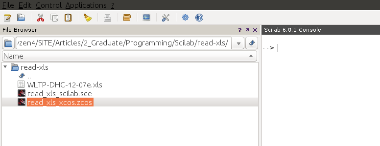
If you are dealing with a lot of data stored in an *.xls file and want to use it in Scilab or Xcos, there is an easy way to import it.
There is predefined Scilab function which can read the content of *.xls files. The Scilab function xls_read() reads a sheet from an Excel file and saves the data in the Scilab workspace. The xls_read() function reads an Excel sheet given a logical unit on an Excel stream and the position of the beginning of the sheet within this stream. It returns the numerical data and the strings contained by the Excel cells.
The read_xls() function can be used to read all sheets from an Excel file in one function with a single function call.
The function can be called as:
[Value,TextInd] = xls_read(fd,Sheetpos)
where:
fd – a number: the logical unit on the Excel stream returned by xls_open() Scilab function
Sheetpos – a number: the position of the beginning of the sheet in the Excel stream. This position is one of those returned by xls_open()
Value – a matrix of numbers: the numerical data found in the sheet. The cells without numerical data are represented by NaN values
TextInd – a matrix of indices with the same size as Value. The 0 indices indicates that no string exists in the corresponding Excel cell. A positive index i points to the string SST(i) where SST is given by xls_open()
Observation: Only BIFF8 Excel files (last Excel file version (2003)) are handled.
Example: Let’s import the data describing the WLTP speed profile. The file can be found here:
http://www.unece.org/fileadmin/DAM/trans/doc/2012/wp29grpe/WLTP-DHC-12-07e.xls
The data will be first imported into Scilab, stored into a variable, and used later in Xcos for simulation purposes.
Step 1. Save the *.xls file in the current Scilab working folder
This way the *.xls file will be found by the xls_open() and xls_read() functions. In this example, the file which is going to be imported is named WLTP-DHC-12-07e.xls.
Step 2. Open the *.xls file and examine the data you want to import. In this example, the data is located in the second sheet, named WLTC_class_3. We will import the WLTP speed profile, which consist of time values and speed values. The time values, in s, begin in the 8th row and 3rd column (C), with value 0. The speed values, in kph, begin in the 8th row and 5th column (E), with value 0.0. If you scroll down towards the end of the table, you’ll see that the last data points are in the row 1808.
Step 3. Open SciNotes and create a script file with the following content:
clear()
clc()
//Decode ole file, extract and open Excel stream
[fd,SST,Sheetnames,Sheetpos] = xls_open('WLTP-DHC-12-07e.xls');
//Read second data sheet
[Value,TextInd] = xls_read(fd,Sheetpos(2));
//close the spreadsheet stream
mclose(fd);
//load WLTP time and speed values in structure
WLTP.time = Value(8:1808,3);
WLTP.values = Value(8:1808,5);
//plot WLTP speed profile
plot(WLTP.time,WLTP.values)
xgrid()
xlabel("Time [s]")
ylabel("Vehicle speed [kph]")
title("x-engineer.org")
The file is opened with the Scilab function xls_open(). The data from the second sheet, Sheetpos(2), is read by the xls_read() function and assigned to the Value variable. Further, the WLTP time and speed values are assigned to the WLTP structure.
Notice that from the variable Value we extracted the data between rows 8 and 1808 and columns 3 and 5, as described in Step 2.
Save the Scilab script as *.sce file in the same Scilab folder.
Step 4. Run the Scilab script and visualise the data.
After running the script we’ll get the following graphical image:
As you can see, the data has been correctly imported, all 1800 time and speed values being plotted.
Step 5. Open Xcos and import the WLTP data from the Scilab workspace
There are two ways of using Scilab data in Xcos simulation:
- by using
From workspaceblock - by using
InterpandTimesource block
In the From workspace block the Variable name is setup as WLTP. The Clock block has the Period set to 1 and Initialisation Time set to 0. The Scope block has the Ymin parameter set to 0, Ymax set to 130, Refresh period and Buffer size are set to 1800.
During the simulation, depending on the simulation time, the right speed value is output from the From workspace block.
Observation: There is a warning message displayed during simulation which is linked to the port sizes. By clicking OK on both warning messages the simulation will be performed.
The second option uses the WLTP data as a look-up table, with the time values as the x-axis and speed values as y-axis. During the simulation, function of the current simulation time, the right speed value is output.
The Time block has no setup parameters. The Interp block has the Xcoord. value set to WLTP.time and the Y coord. parameter set to WLTP.values. The Clock and Scope parameters are the same as in the first example.
Step 6. Run the Xcos simulation.
Set the Simulation -> Setup, Final integration time parameter to 1800 and run simulation. In both examples, the folowing graphical image will be generated:
This confirms that the data was correctly imported from the Scilab workspace.
This method can be easily used to import any kind of *.xls data into Scilab and Xcos, and used into further simulation applications. Just make sure you have the required files in the Scilab work folder and setup correctly the import parameters.


Shimin V V
Very useful and nicely explained.